THOMPSON SAMPLING
Beta distribution
Thompson sampling을 설명할 때 sampling distribution update과정을 beta-binomial distribution로 설명하기가 쉬우므로 많이 쓴다.
먼저 beta distribution의 probability density function은 다음과 같다.
\(Beta(\theta,\alpha,\beta) = \frac{\Gamma(\alpha + \beta)}{\Gamma(\alpha)\Gamma(\beta)}\theta^{\alpha -1}(\theta-1)^{\beta -1}\)
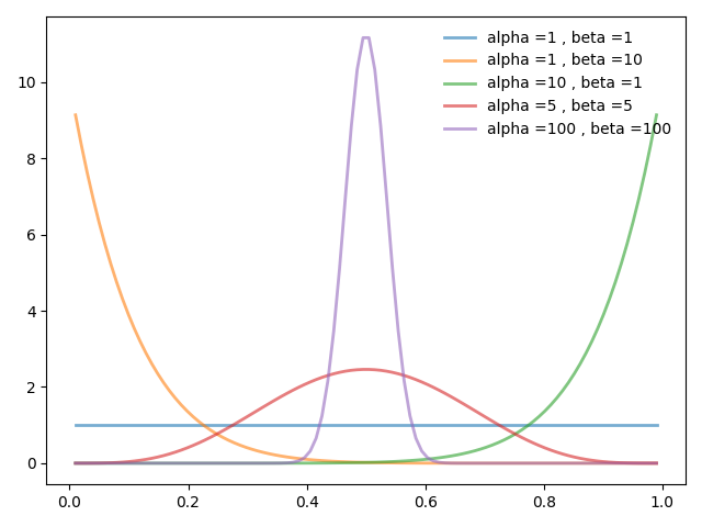
그림 1. Beta distribution
예시 그림에서와 같이 $\alpha$값이 상대적으로 높을수록 positive skew된, $\beta$값이 상대적으로 높을수록 negative skew된 것을 볼 수 있다.
그리고 $\alpha$와 $\beta$값 높을 수록 좌우가 분포가 peak이 높은 형태를 나타내는 것도 확인 할 수 있다.
Gamma function
Beta distribution의 gamma function은 다음과 같은 형태를 가지고 있다. \(\Gamma(\alpha) = \int_{0}^{\infty} t^{\alpha - 1} e^{-t} dt\)
Intgeration by parts를 적용하여 풀어주면,
$ \int_{0}^{\infty} t^{\alpha - 1} e^{-t} dt $
$=-t^{\alpha - 1}e^{-t} \bigg\rvert_{t=0}^{\infty} + \int_{0}^{\infty} (x-1)t^{\alpha -2}e^{-t} dt$
$= 0 + \int_{0}^{\infty} (x-1)t^{\alpha -2}e^{-t} dt$
$=(x-1)\Gamma(x-2)$
이 방법을 연속적으로 취해주면 $ \Gamma (x) = (x-1)! $임을 알 수 있다.
Beta-binomial distribution
위의 두 사실을 바탕으로 다음과 같은 등식이 성립한다.
\[{\frac{\Gamma(\alpha + \beta)}{\Gamma(\alpha)\Gamma(\beta)}\theta^{\alpha -1}(\theta-1)^{\beta -1} = \frac{(\alpha+\beta -1)!}{(\alpha-1)!(\beta-1)!}\theta^{\alpha-1}(\theta-1)^{\beta-1}}\]다음으로 위의 사실이 어떻게 Binomial distribution과 연관되는지 알아보도록 하자.
Bayesian update for binomial distribution
binomial distribution은 bernoulli distribution이라고도 부르고 probability density function은 다음과 같이 정의된다.
\(bin(n,k,\theta) = \binom{n}{k}\theta^{k}(\theta-1)^{n-k}\)
, where $\theta$ = probability of success, $k$ = trial of sucess
Binomial distribution에서 posterior를 계산하는 방법은 다음과 같다.
$p(\theta \mid x) = \frac{p(x \mid \theta)p(\theta)}{p(x)}$, we assume that $p(\theta)$ = 1
$= \frac{\binom{n}{k}\theta^{k}(\theta-1)^{n-k}}{\binom{n}{k}\int_{\theta}\theta^{k}{(\theta-1)}^{n-k}d\theta}$
$= \frac{\theta^{k}(\theta-1)^{n-k}}{\frac{\Gamma(k+1)\Gamma(n-k+1)}{\Gamma(n+2)}}$
$= \frac{\Gamma(n+2)}{\Gamma(k+1)\Gamma(n-k+1)}\theta^{k}(\theta-1)^{n-k}$
$= Beta(\theta,k+1,n-k+1)$
따라서 $bin(n,k)$의 posterior는 $Beta(k+1,n-k+1)$과 같다.
Bayesian update for beta-binomial distribution
만약 prior $p(\theta)$가 beta distribution을 다른다고 가정하면 어떻게 될까?
bayesian inference
bayesian inference에서는 계산의 복잡성에 의해 normalizing constant (여기서는 $p(x)$)를 생략하기도 한다. 따라서 다음과 같은 식이 된다.
\[posterior \propto likelihood \ast prior\]따라서 posterior는 다음과 같이 구해진다.
$p(\theta \mid x) \propto p(x \mid \theta)p(\theta)$, we assume that $p(\theta) = Beta(\alpha,\beta)$
$\approx \binom{n}{k}\theta^{k}(\theta-1)^{n-k}\frac{\Gamma(\alpha + \beta)}{\Gamma(\alpha)\Gamma(\beta)}\theta^{\alpha -1}(\theta-1)^{\beta -1}$
$\approx \binom{n}{k}\frac{\Gamma(\alpha + \beta)}{\Gamma(\alpha)\Gamma(\beta)}\theta^{k+\alpha -1}(\theta-1)^{n-k+\beta -1}$
$\approx Beta(x+\alpha, n-x+\beta)$
Tompson sampling for bernoulli bandit
bandit problem을 이야기할 때에 보통 슬롯머신 비유를 많이한다. 간단하게 이야기하면 여러개의 슬롯머신이 있고 그 중 어떤 슬롯머신의 손잡이를 잡아 당겼을 때 돈을 확률이 높은지를 고민하는 문제라고 할 수 있겠다.
아래의 알고리즘은 bandit problem 최적의 선택(어떤 슬롯머신의 손잡이를 당겼을 때 돈을 딸 확률이 높은지)을 구하는 알고리즘이다.
Psudo-code for bernoulli thompson sampling
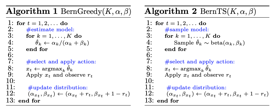
그림 2. Bernoulli greedy algorithm(좌) Bernoulli thompson sampling algorithm(우)
두 알고리즘의 가장 주요한 차이는 전자는 $\hat{\theta_{k}}$값을 구할 때 mean값 사용하고 후자는 beta distribution에 의해 분포된 probability density에 따라 확률이 랜덤하게 선택된다는 것이다.
Algorithm2에 대한 해설
$t$는 trial에 대한 index이고 $k$는 choice에 대한 index를 나타낸다.
$t$번째 trial에서 각 choice에 대한 ${\theta_{k}}$값들(다르게 말해 성공확률들)이 구해질 것이고, 이 확률들 중 가장 높은 확률을 가지는 $\theta_{k}$를 $\hat{\theta_{k}}$로 선택한다.
가장 큰 성공확률을 나타내는 $\hat{\theta_{k}}$가 선택 되었으면 $\hat{\theta_{k}}$에 대응되는 choice를 $x_{t}$로 두고 이에 대한 reward값인 $r_{t}$ 확인한다.
Bayesian inference를 적용해 reward값 $r_{t}$를 parameter로 하는 $Beta(r_{t},r_{t}-1)$을 prior로 두고 posterior를 구$Beta(\alpha+r,\beta+r-1)$가 된다.
앞서 그림 1을 통해 beta distribution의 분포특성을 살펴봤듯이 두 파라미터 값($\alpha$, $\beta$)값이 높아질 수록 분포의 폭이 좁아지는 경향을 보인다.
그리고 알고리즘의 trial이 높아 질수록 이 두 파라미터 값이 증가한다.
즉, ${\theta_{k}}$의 sampling distribution의 variance가 작아진다. 따라서 랜덤하게 추출되는 ${\theta_{k}}$값이 균질해진다.
그리고, 이러한 효과는 높은 성공확률을 가지는 분포에서 random sampling한 ${\theta_{k}}$의 값이 균질 (또는 명백히 하는) 효과를 준다.
$\epsilon$-greedy algorithm에서는 $\epsilon$값에 의해 성공확률 이외에도 랜덤하게 다른 choice를 할 여지는 주지만 성공확률이 확연히 차이나는 선택이 존재할 경우 이러한 방식은 도움이 되지 않는다.
reference : https://web.stanford.edu/~bvr/pubs/TS_Tutorial.pdf